Review of linear models, probability distributions
Assigned Reading:
- Guthery, Fred S., and Ralph L. Bingham. “A primer on interpreting regression models.” The Journal of Wildlife Management 71.3 (2007): 684-692.
- Chapter 3 of Hobbs, N. T., & Hooten, M. B. (2015). Bayesian models: a statistical primer for ecologists. Princeton University Press.
Overview
We will be reviewing linear models (linear regression) using the Palmer Penguins dataset and R Package. We will start with generating hypotheses, then move on to data exploration, fitting our first model, checking that our model fits linear regression assumptions, and finally interpreting our model. Please download this R script. We will work through it as we go through the examples and challenges below.
Meet the penguin species that we’ll be working with:

Here’s the packages and data
# List of packages necessary to run this script:
require(librarian, quietly = TRUE)
shelf(tidyverse, cowplot, palmerpenguins, performance, bslib, shiny,
      ggExtra,
      quiet = TRUE)

# # Here is the link to the R Package with the penguins data:
# https://allisonhorst.github.io/palmerpenguins/

# Read in a data file
data(package = 'palmerpenguins',
     verbose = FALSE)
Take a look at the data. The head() function is good for this. On your own, try the str() function on the entire data.frame, the range() function on individual numeric columns, and the unique() function on character columns.
Note: there are two datasets included in the “palmerpenguins” package. We will use the cleaned ‘penguins’ dataset.
head(penguins)## # A tibble: 6 × 8
## species island bill_length_mm bill_depth_mm flipper_length_mm body_mass_g
## <fct> <fct> <dbl> <dbl> <int> <int>
## 1 Adelie Torgersen 39.1 18.7 181 3750
## 2 Adelie Torgersen 39.5 17.4 186 3800
## 3 Adelie Torgersen 40.3 18 195 3250
## 4 Adelie Torgersen NA NA NA NA
## 5 Adelie Torgersen 36.7 19.3 193 3450
## 6 Adelie Torgersen 39.3 20.6 190 3650
## # ℹ 2 more variables: sex <fct>, year <int>Try out some data exploration techniques that we’ve learned. Here, I’ve plotted histograms of body mass by species by island. On your own, look for outliers, make scatterplots, and whatever else you want to try.
## Warning: Removed 2 rows containing non-finite outside the scale
## range (`stat_bin()`).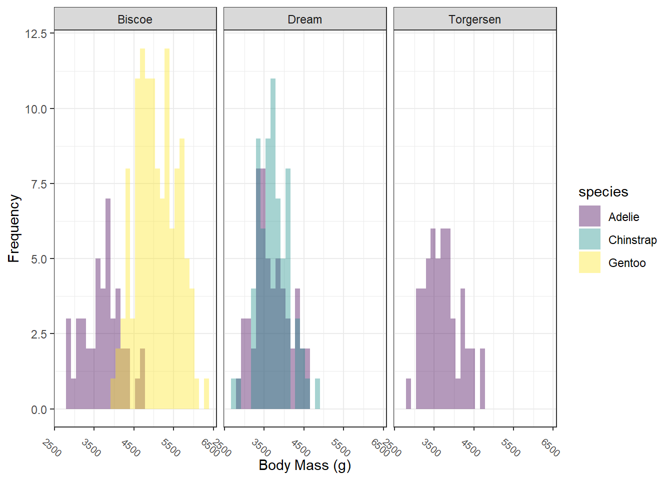
Let’s try a model!
A pretty reasonable hypothesis to test is “In penguins, males will have greater body mass than females, and body mass is also allometrically related to bill length and depth.” We could also add that “body mass will vary across species.”
To test this hypothesis, let’s create a ‘global’ model containing all the variables that our hypotheses predict will influence body mass:
# fit the global linear regression
fit_global <-
  lm(body_mass_g ~ sex + bill_length_mm * bill_depth_mm + species,
     data = penguins)

# Check out the global model's coefficients, R^2 values, and p-values.
summary(fit_global)
##
## Call:
## lm(formula = body_mass_g ~ sex + bill_length_mm * bill_depth_mm +
## species, data = penguins)
##
## Residuals:
## Min 1Q Median 3Q Max
## -787.41 -179.56 -6.98 199.41 904.99
##
## Coefficients:
## Estimate Std. Error t value Pr(>|t|)
## (Intercept) -3184.722 1833.850 -1.737 0.08340 .
## sexmale 440.126 48.824 9.014 < 2e-16 ***
## bill_length_mm 121.948 42.986 2.837 0.00484 **
## bill_depth_mm 315.022 102.849 3.063 0.00237 **
## speciesChinstrap -201.897 86.241 -2.341 0.01983 *
## speciesGentoo 1379.565 110.804 12.451 < 2e-16 ***
## bill_length_mm:bill_depth_mm -5.386 2.392 -2.251 0.02503 *
## ---
## Signif. codes: 0 '***' 0.001 '**' 0.01 '*' 0.05 '.' 0.1 ' ' 1
##
## Residual standard error: 298 on 326 degrees of freedom
## (11 observations deleted due to missingness)
## Multiple R-squared: 0.8655, Adjusted R-squared: 0.8631
## F-statistic: 349.7 on 6 and 326 DF, p-value: < 2.2e-16We did it! Go line-by-line through the summary table and–in words–communicate if each hypothesis is supported and why.
Additionally, you may be asking a common question for folks using categorical variables in regression. In this case, it’s probably “why are there no coefficient estimates for sex:female or species:Adelie?” On your own, search Google and/or StackOverflow for an answer.
Collinearity?
But wait–we forgot a critical step: checking for collinearity in the predictor variables! Now that we have a fitted model, we can use VIFs to assess collinearity:
# Use performance::check_collinearity to calculate VIFs:
check_collinearity(fit_global)
## Model has interaction terms. VIFs might be inflated.
## Try to center the variables used for the interaction, or check
## multicollinearity among predictors of a model without interaction terms.## # Check for Multicollinearity
##
## Low Correlation
##
## Term VIF VIF 95% CI adj. VIF Tolerance Tolerance 95% CI
## sex 2.23 [ 1.92, 2.66] 1.49 0.45 [0.38, 0.52]
##
## High Correlation
##
## Term VIF VIF 95% CI adj. VIF Tolerance
## bill_length_mm 206.62 [167.80, 254.47] 14.37 4.84e-03
## bill_depth_mm 153.38 [124.59, 188.87] 12.38 6.52e-03
## species 28.03 [ 22.85, 34.43] 2.30 0.04
## bill_length_mm:bill_depth_mm 287.47 [233.43, 354.09] 16.96 3.48e-03
## Tolerance 95% CI
## [0.00, 0.01]
## [0.01, 0.01]
## [0.03, 0.04]
## [0.00, 0.00]Uh oh. Looks like we have >>> 10 VIFs for all predictor variables except sex! Are our species and allometric hypotheses scuppered?!
Before we get too morose, let’s try a few things to double-check these VIFs are giving us accurate information. First, it stands to reason that if we have interaction terms such as ‘x’, ‘y’ and ‘xy,’ then ‘x’ and ‘y’ will be correlated with their product ‘xy,’ right? One way to demonstrate this is by standardizing (i.e., centering or scaling) the offending numeric predictor variables and recalculating VIFs. This should reduce the collinearity at least for the interaction terms. Let’s try it:
# Create a new data.frame with
penguins <-
  penguins %>%
  mutate(across(c(bill_length_mm, bill_depth_mm),
                .fns = function(X) as.numeric(scale(X)),
                .names = "{.col}_scaled"))

# fit the global linear regression
fit_global_scaled <-
  lm(body_mass_g ~ sex + bill_length_mm_scaled * bill_depth_mm_scaled + species,
     data = penguins)

# Use performance::check_collinearity to calculate VIFs:
check_collinearity(fit_global_scaled)
## Model has interaction terms. VIFs might be inflated.
## Try to center the variables used for the interaction, or check
## multicollinearity among predictors of a model without interaction terms.## # Check for Multicollinearity
##
## Low Correlation
##
## Term VIF VIF 95% CI adj. VIF
## sex 2.23 [ 1.92, 2.66] 1.49
## bill_length_mm_scaled:bill_depth_mm_scaled 1.75 [ 1.53, 2.07] 1.32
## Tolerance Tolerance 95% CI
## 0.45 [0.38, 0.52]
## 0.57 [0.48, 0.65]
##
## Moderate Correlation
##
## Term VIF VIF 95% CI adj. VIF Tolerance Tolerance 95% CI
## bill_length_mm_scaled 6.00 [ 4.97, 7.29] 2.45 0.17 [0.14, 0.20]
## bill_depth_mm_scaled 6.11 [ 5.07, 7.43] 2.47 0.16 [0.13, 0.20]
##
## High Correlation
##
## Term VIF VIF 95% CI adj. VIF Tolerance Tolerance 95% CI
## species 28.03 [22.85, 34.43] 2.30 0.04 [0.03, 0.04]Okay, so far so good. The second thing to check is whether coefficient, p-values, and \(R^2\) values have changed between the un-standardized global model and the standardized global model. Run this block on your own and see what happens:
# Compare coefficients and p-values.
summary(fit_global)$coefficients # Note: summary() creates a list that you can index for specific model information.
summary(fit_global_scaled)$coefficients

# Compare R^2 values
summary(fit_global)$adj.r.squared
summary(fit_global_scaled)$adj.r.squared
Great! Both our expectations for the interaction terms were confirmed, and we don’t need to worry about high VIFs there.
However, we still need to deal with the > 10 VIF for species, which does appear to be accurate. Fortunately, the answer is simple: drop the species variable from the model and recheck for collinearity. On your own, consider model outputs from the code chunk below and compare these to previous model outputs:
# fit the global linear regression
fit_global_scaled_noSpecies <-
  lm(body_mass_g ~ sex + bill_length_mm_scaled * bill_depth_mm_scaled,
     data = penguins)

# Check collinearity
check_collinearity(fit_global_scaled_noSpecies)
## # Check for Multicollinearity
##
## Low Correlation
##
## Term VIF VIF 95% CI adj. VIF
## sex 1.65 [1.45, 1.94] 1.28
## bill_length_mm_scaled 1.69 [1.48, 1.99] 1.30
## bill_depth_mm_scaled 1.63 [1.43, 1.91] 1.28
## bill_length_mm_scaled:bill_depth_mm_scaled 1.29 [1.17, 1.52] 1.14
## Tolerance Tolerance 95% CI
## 0.61 [0.52, 0.69]
## 0.59 [0.50, 0.67]
## 0.61 [0.52, 0.70]
## 0.77 [0.66, 0.86]# Check out the global model's coefficients, R^2 values, and p-values.
summary(fit_global_scaled_noSpecies)##
## Call:
## lm(formula = body_mass_g ~ sex + bill_length_mm_scaled * bill_depth_mm_scaled,
## data = penguins)
##
## Residuals:
## Min 1Q Median 3Q Max
## -1382.55 -264.66 -9.64 246.14 1268.04
##
## Coefficients:
## Estimate Std. Error t value Pr(>|t|)
## (Intercept) 3755.42 35.23 106.612 <2e-16
## sexmale 770.97 57.12 13.497 <2e-16
## bill_length_mm_scaled 313.58 28.95 10.832 <2e-16
## bill_depth_mm_scaled -411.92 28.51 -14.446 <2e-16
## bill_length_mm_scaled:bill_depth_mm_scaled -270.09 30.19 -8.946 <2e-16
##
## (Intercept) ***
## sexmale ***
## bill_length_mm_scaled ***
## bill_depth_mm_scaled ***
## bill_length_mm_scaled:bill_depth_mm_scaled ***
## ---
## Signif. codes: 0 '***' 0.001 '**' 0.01 '*' 0.05 '.' 0.1 ' ' 1
##
## Residual standard error: 406.2 on 328 degrees of freedom
## (11 observations deleted due to missingness)
## Multiple R-squared: 0.7486, Adjusted R-squared: 0.7455
## F-statistic: 244.2 on 4 and 328 DF, p-value: < 2.2e-16Model diagnostics
As a last step, we need to make sure our final model meets all required assumptions for a linear regression:
- Linear relationship between response and predictor variables
- Reasonable levels of collinearity (e.g., VIF < 3 or 5 or 10)
- Homogeneity of variances between groups (i.e., homoscedasticity [i.e., NOT heteroscedasticity])
- Errors are normally distributed
- Independent sampling (i.e., no autocorrelation or pseudoreplication)
We’ve already dealt with collinearity, we know there is a linear relationship between response and predictor variables. On your own, go back through our previous work to determine where and how we checked for collinearity and the linear relationship–and what the outcomes were.
We will wait until our Autocorrelation topic to check for independence, but we let’s definitely check for homogeneity of variances and normal error distributions:
# Check for heteroscedasticity via the fancy ggplot2 way of plotting fitted values vs. residuals:
ggplot() +
  geom_point(aes(x = fit_global_scaled_noSpecies$fitted.values,
                 y = fit_global_scaled_noSpecies$residuals)) +
  geom_hline(data = data.frame(yintercept = 0),
             aes(yintercept = 0),
             linetype = 2,
             color = "red") +
  xlab("Fitted values") +
  ylab("Residuals")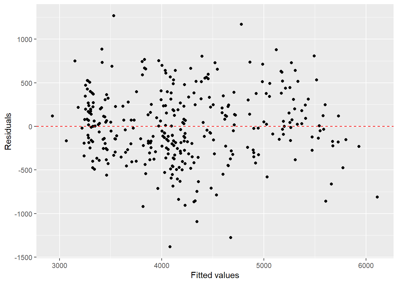
# Built-in model diagnostics for checking for heteroscedasticity, errors are normally distributed, etc.
par(mfrow = c(2, 2)) # To make all plots be panels of a single figure.
plot(fit_global_scaled_noSpecies)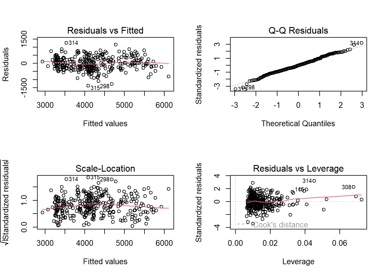
So our final model contains sex and an interaction of bill length and depth to explain body mass in penguins. We’ve successfully created our first linear model!
Visualizations and Predictions
One last thing: we should make some visualizations of our model outputs.
Dotplots
We don’t want stop at the model summary table: we need to visualize the model outputs. This is critical for publications, reports, science communication, and just helping us understand the model. We also need to be honest about the uncertainty (variation) in our estimates.
First of all, let’s make some dot-and-whisker plots to display our coefficient estimates and uncertainty (i.e., confidence intervals). We’ll need to extract the coefficient estimates and calculate confidence intervals.
There are multiple ways to extract coefficient estimates
coef(fit_global_scaled_noSpecies) # Just coefficient estimates## (Intercept)
## 3755.4151
## sexmale
## 770.9732
## bill_length_mm_scaled
## 313.5795
## bill_depth_mm_scaled
## -411.9157
## bill_length_mm_scaled:bill_depth_mm_scaled
## -270.0916summary(fit_global_scaled_noSpecies)$coefficients # whole model table. It's a matrix, so you can index!## Estimate Std. Error t value
## (Intercept) 3755.4151 35.22500 106.612200
## sexmale 770.9732 57.12296 13.496730
## bill_length_mm_scaled 313.5795 28.94864 10.832271
## bill_depth_mm_scaled -411.9157 28.51419 -14.445989
## bill_length_mm_scaled:bill_depth_mm_scaled -270.0916 30.19029 -8.946308
## Pr(>|t|)
## (Intercept) 1.277010e-256
## sexmale 2.536182e-33
## bill_length_mm_scaled 1.405624e-23
## bill_depth_mm_scaled 5.968268e-37
## bill_length_mm_scaled:bill_depth_mm_scaled 2.759474e-17summary(fit_global_scaled_noSpecies)$coefficients[ , 1] # First column is just coefficient estimates.## (Intercept)
## 3755.4151
## sexmale
## 770.9732
## bill_length_mm_scaled
## 313.5795
## bill_depth_mm_scaled
## -411.9157
## bill_length_mm_scaled:bill_depth_mm_scaled
## -270.0916summary(fit_global_scaled_noSpecies)$coefficients[ , 2] # Second column is standard error estimates.## (Intercept)
## 35.22500
## sexmale
## 57.12296
## bill_length_mm_scaled
## 28.94864
## bill_depth_mm_scaled
## 28.51419
## bill_length_mm_scaled:bill_depth_mm_scaled
## 30.19029For all models that use the normal (Gaussian) distribution and the “identity” link function, confidence intervals are very easy to estimate:
- Step 1: Find a t-score table and look for your desired level of confidence.
- Step 2: Multiply the t-score by the Standard Error estimate.
- Step 3: Subtract/Add the product from the coefficient estimate for the upper/ lower confidence limit.
Here’s a by-hand example for 95% confidence. NOTE: 95% confidence means the interval ranges from 2.5% - 97.5%. Why?
# Make a data.frame with the coefficient estimates and confidence intervals
dotplot_df <-
  data.frame(CI_0.975 = coef(fit_global_scaled_noSpecies) + ((summary(fit_global_scaled_noSpecies)$coefficients[, 2]) * 1.96),
             CI_0.025 = coef(fit_global_scaled_noSpecies) - ((summary(fit_global_scaled_noSpecies)$coefficients[, 2]) * 1.96),
             CoefEsts = coef(fit_global_scaled_noSpecies),
             CoefNames = c("Intercept", "Sex-Male", "Bill Length", "Bill Depth",
                           "Bill Length:Bill Depth")
  )

# Make a dotplot!
ggplot(dotplot_df %>%
         # Removing intercept because we usually don't include them in dotplots
         filter(CoefNames != "Intercept"),
       aes(x = CoefNames,
           y = CoefEsts,
           ymin = CI_0.025,
           ymax = CI_0.975)) +
  geom_point(size = 2) +
  geom_errorbar(width = 0.1) +
  geom_hline(data = data.frame(yintercept = 0),
             mapping = aes(yintercept = yintercept),
             linetype = 2,
             color = "darkred") +
  theme_bw() +
  ylab("Coefficient Estimate") +
  xlab("Coefficient Names")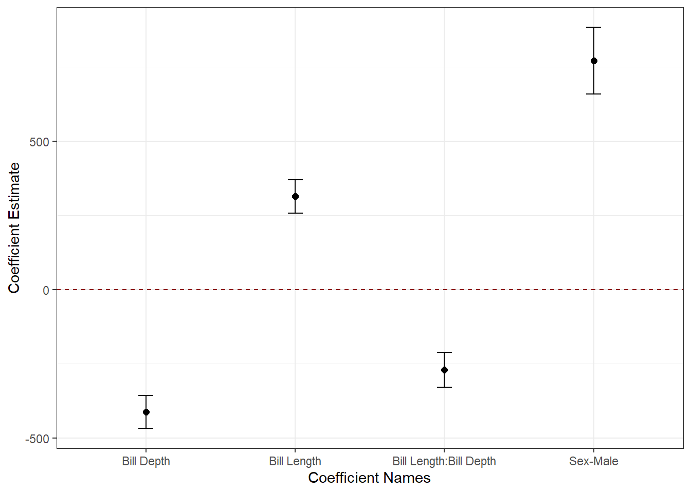
Effect plots
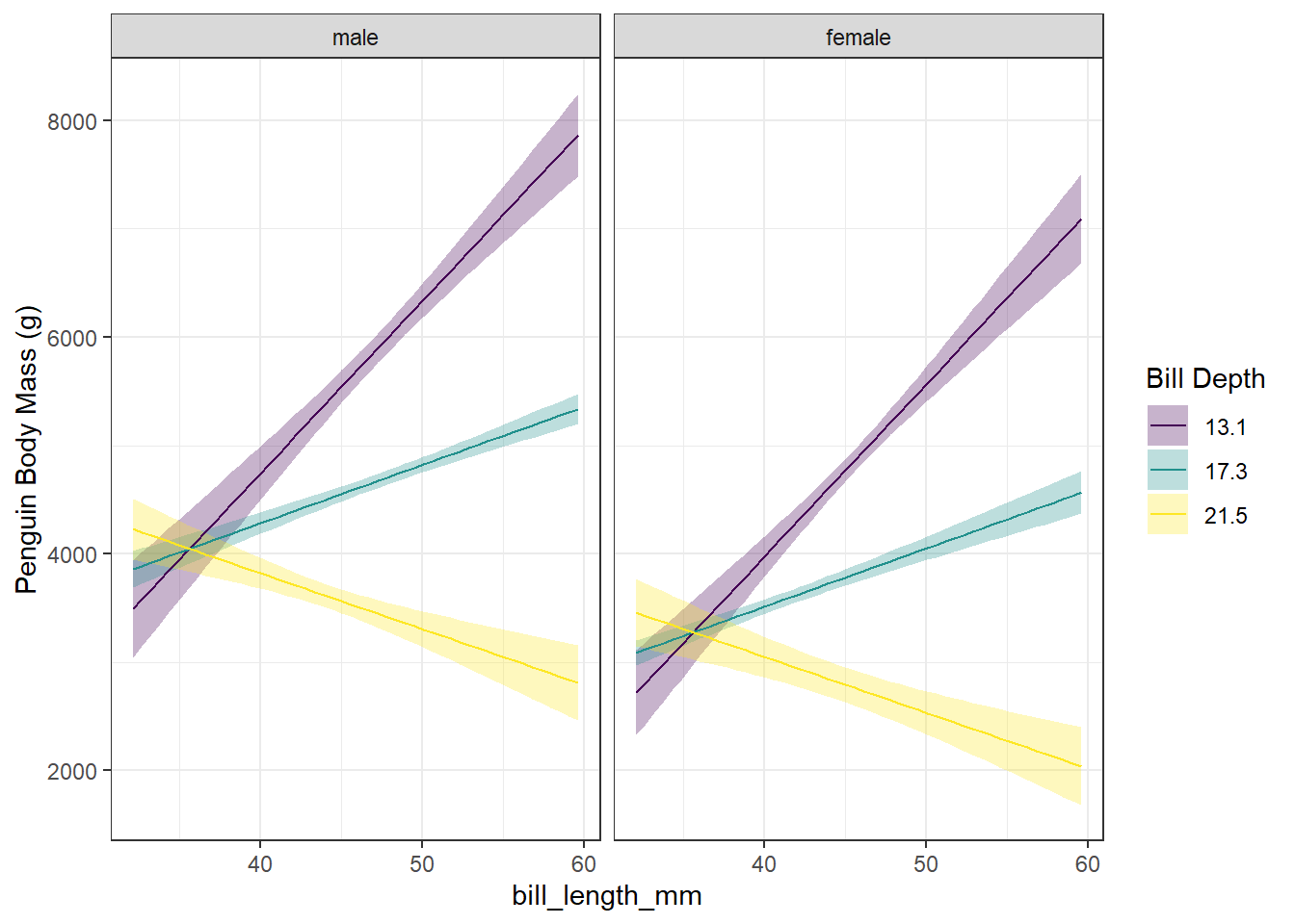
Dotplots are fantastic, but showing trend lines can be even more powerful. This can get a little tricky when there are multiple covariates–especially when there are interactions. It can also be hard to interpret an interactive effect just from dotplots. Let’s create effects plots with the interactive effects.
Here’s the general workflow:
- Step 1: Create a “new” data.frame with ranges of predictor variable values on which to make predictions. NOTE: I strongly suggest you constrain the ranges to the range of the data to avoid the perils of extrapolation.
- Step 2: Use the model fit to predict response variable estimates and standard errors at the predictor variable values in the new data.frame.
- Step 3: Calculate confidence intervals.
- Step 4: Plot the estimated responses + confidence intervals
Let’s start by using the handy “expand.grid” function to create the new data.frame. Where there are empty comments below, annotate with what the code is doing:
# Create a data.frame for predictions
nd <-
  #
  with(penguins,
       #
       expand.grid(
         #
         sex = c("male", "female"),
         #
         bill_length_mm = seq(min(bill_length_mm, na.rm = TRUE),
                              max(bill_length_mm, na.rm = TRUE),
                              #
                              length.out = 50),
         #
         bill_depth_mm = c(min(bill_depth_mm, na.rm = TRUE),
                           median(bill_depth_mm, na.rm = TRUE),
                           max(bill_depth_mm, na.rm = TRUE)))
  )

# Add scaled covariates. NOTE: You have to use the ORIGINAL mean and SD from the ORIGINAL dataset.
nd_new <-
  nd %>%
  mutate(bill_length_mm_scaled = as.numeric((bill_length_mm - mean(penguins$bill_length_mm, na.rm = T)) /                     sd(penguins$bill_length_mm, na.rm = T)),
         bill_depth_mm_scaled = as.numeric((bill_depth_mm - mean(penguins$bill_depth_mm, na.rm = T)) /                       sd(penguins$bill_depth_mm, na.rm = T)))

# Predict and calculate confidence intervals
pred_df <-
  data.frame(nd_new,
             as.data.frame(predict(fit_global_scaled_noSpecies, nd_new, se.fit = TRUE))) %>%
  mutate(CI_0.975 = fit + (se.fit * 1.96),
         CI_0.025 = fit - (se.fit * 1.96))

# Plot the effects!
ggplot(pred_df,
       aes(x = bill_length_mm,
           y = fit,
           color = as.factor(bill_depth_mm),
           fill = as.factor(bill_depth_mm),
           group = as.factor(bill_depth_mm),
           ymin = CI_0.025,
           ymax = CI_0.975)) +
  facet_wrap(~ sex) +
  geom_ribbon(alpha = 0.3,
              color = NA) +
  geom_line() +
  scale_colour_viridis_d(name = "Bill Depth") +
  scale_fill_viridis_d(name = "Bill Depth") +
  theme_bw() +
  ylab("Penguin Body Mass (g)")