Homework 4
Overview
Please provide a reproducible .Rmd script to address the scenario below and produces all of your analysis and plots. Some reminders:
- Reproducible: This means when I run your .Rmd file, it will run all analyses and create all plots without errors, without me having to reset my working directory, and without forcing me to install anything on my machine (i.e., use the require(librarian); shelf(your packages, lib = tempdir()) approach as in the code block below). This also means there should be NO ERRORS when I run it!
- Format: In the .Rmd file, arrange and format similar to a scientific article. Specifically, I want to see 1) an analytical methods section, 2) a results section that includes figures, tables, and text interpreting the figures and tables and model(s)!, and 3) a brief conclusion (1 - 2 paragraphs) based on the results. NOTE: You do not need to create an introduction, reiterate the data collection methods, or produce a literature cited section!
Background

In the face of woody plant encroachment, prescribed fire is an essential management tool for maintaining grassland ecosystems in the North American Great Plains. To safely and efficiently conduct prescribed fires, land managers often try to burn only under narrow weather conditions. For example, it can be unsafe to burn when the relative humidity (RH) is too low, and fires can be less effective in controlling woody plants if the humidity is too high. Likewise, fires can move too quickly and get out of control if wind speeds are too fast, but the fire may not move across the landscape if there is no wind at all.
Climate change stands to further complicate the use of prescribed fire. Climate change may cause longer and more severe droughts and wind speeds may increase or become more erratic. To understand and adjust fire prescriptions under climate change–while still putting fire on landscapes to control woody plant encroachment–managers need to understand how current weather factors change across years, individual burn seasons, and across the extent of the Great Plains.
Data description
To address this need, you will be using weather station data collected across a latitudinal gradient in the US Great Plains. The weather station data was collected from 2010 - 2019 and between days 121 - 273 in each year (roughly May - September). Descriptions of data in each column are as follows:
| Column Name | Description |
|---|---|
| Year | years 2010 - 2019 |
| Veg_Type | vegetation type/ecoregion in which the weather station falls |
| Station_ID | unique identifier for each weather station |
| Lat | latitude |
| Long | longitude |
| Month | numeric month of year (e.g., 5 = May) |
| Day | |
| Wind_mph_max | maximum daily wind speed in miles per hour |
| RH_per_min | minimum daily relative humidity as a percent |
Your assignment
Use hierarchical generalized additive models to characterize daily minimum RH and daily maximum wind speeds. Specifically, you will be answering this question:
How do the two weather metrics of interest (minimum RH and maximum wind speed) change over time and across space?
You will need to decide what statistical distributions to use, how to structure the “hierarchical” part of the models, etc. Use the Pederson et al. (2019) manuscript to help make modeling and figure creation decisions!
# List of packages necessary to run this script:
require(librarian, quietly = TRUE)
shelf(tidyverse,
      maps, # For US state map
      mgcv, # For checking model convergence
      MuMIn, # for model selection
      gratia, # for ggplot functionality with mgcv
      sf,
      lib = tempdir(),
      quiet = TRUE)

# Set the web address where R will look for files from this repository
# Do not change this address
repo_url <- "https://raw.githubusercontent.com/LivingLandscapes/Course_EcologicalModeling/master/"

# Load data
weather <-
  read_csv(paste0(repo_url, "data/FireWeather.csv"))

# Brief looks at the data:
head(weather)
## # A tibble: 6 × 9
## Year Veg_Type Station_ID Lat Long Month Day Wind_mph_max RH_per_min
## <dbl> <chr> <chr> <dbl> <dbl> <dbl> <dbl> <dbl> <dbl>
## 1 2010 Edwards Plat… KGRK 31.1 -97.8 5 121 17.3 40.9
## 2 2010 Edwards Plat… KGRK 31.1 -97.8 5 122 16.1 26.3
## 3 2010 Edwards Plat… KGRK 31.1 -97.8 5 123 11.5 24.8
## 4 2010 Edwards Plat… KGRK 31.1 -97.8 5 124 11.5 20.9
## 5 2010 Edwards Plat… KGRK 31.1 -97.8 5 125 13.8 31.8
## 6 2010 Edwards Plat… KGRK 31.1 -97.8 5 126 19.6 38.0# Convert to an sf object for mapping
weather_sf <- st_as_sf(weather,
crs = st_crs(4326),
coords = c("Long", "Lat"))
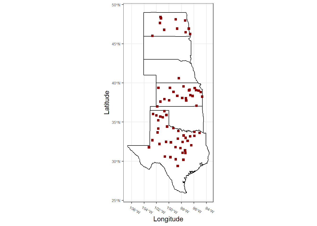
# Get a US states map
states <- map_data("state") # Map of US states
# Make a map to show where the weather stations are:
ggplot() +
geom_polygon(data = states %>% filter(region %in% c("north dakota",
"south dakota",
"nebraska",
"kansas",
"oklahoma",
"texas")),
mapping = aes(x = long, y = lat, group = group),
fill = "white",
color = "black") +
geom_sf(data = weather_sf,
shape = 15,
color = "darkred") +
theme_bw() +
theme(panel.grid.minor = element_blank(),
axis.text.x = element_text(angle = 330),
axis.text = element_text(size = 6,
hjust = 0.1)) +
xlab("Longitude") +
ylab("Latitude")