Bayesian Mixed Models: Choose your own adventure!
Overview
This week, it’s “choose your own adventure” time. I want you to work in pairs to tackle this scenario below:
The data are the weights of deer harvested at Desoto National Wildlife Refuge between 2003 and 2006. Refuge biologists were trying to reduce the population to prevent overbrowsing and damage to the remaining habitat, especially as they convert existing row crops on the refuge to warm season perennial grasses. They were interested in whether the weight of harvested deer decreases when populations are relatively high in the refuge – this is expected because of density dependent reductions in body condition. It’s reasonable to expect deer of different sexes and ages to weigh different amounts – the key question is how much do they vary among years and hunts, and is mass a good indirect indicator of density?
Your task
Develop a Bayesian mixed model provide the refuge biologists an answer to their deer question. Specifically:
- Conduct some data exploration. (15 minutes)
- Formulate/run Bayesian mixed model(s) to answer the question. (20 minutes)
- Check model diagnostics. (10 minutes)
- Create figures to demonstrate model outcomes. (20 minutes)
Work in teams (Dr. Roberts will assign). Dr. Roberts will call on teams to present different stages of the work to the class.

Data description:
Each row in the dataset corresponds to a single deer.
# Load packages
require(librarian)
shelf(brms, cmdstanr, tidyverse,
      lib = tempdir())

# Set the web address where R will look for files from this repository
repo_url <- "https://raw.githubusercontent.com/LivingLandscapes/Course_EcologicalModeling/master/"

# Load the data
deer <-
  read.table(paste0(repo_url, "data/csd2003-2006kg.txt"),
             header=TRUE)

### Data columns
# num – unique identifier of each deer
# location – always “desoto"
# hunt – either “AL” or “ES” – different types of hunt “AntlerLess” or “EitherSex”. Deer should be smaller in the AL hunts because the focus is on deer without Antlers.
# bonus – y or n depending on whether it was a “bonus tag” deer
# num.totaltag – total number of tags for that hunt
# num.tag – number of normal tags issued
# num.bonustag – number of bonus tags issued
# year         month        day – actual date of the hunt
# hunt.year – which “season” was it (i.e. Jan 2005 is part of the 2004 “hunt year”)
# sex – duh.
# Age – numeric estimate of age
# age.class – factor variable for age class (more reliable than age)
# mass - pounds
# kg.mass - kg
# buck.count – an index of the buck population
# doe.count – an index of the doe population
# fawn.count  - an index of the fawn population
# b.d – bucks per doe (estimate of sex ratio)
# f.d – fawns per doe (estimate of productivity)
# ha.crop – hectares of the refuge in row crop
# ha.corn      ha.soybean
# h.count – index of population prior to harvest
# harvest – number harvested
# hpue – harvest per unit effort
# d.est  - estimated  # of deer in the refuge (independent helicopter count)

# Convert age.class to a factor
deer$age.class <- factor(deer$age.class)

# Very briefly explore:
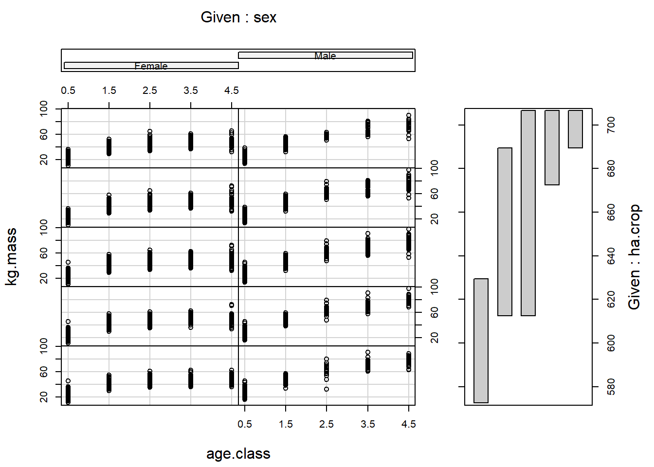
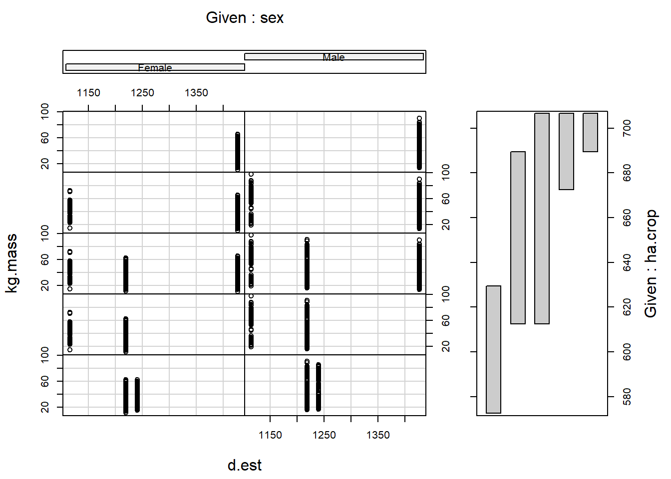
coplot(kg.mass ~ age.class | sex * ha.crop,
data = deer)